How to Leverage Excel Formulas for SEO Success

Do you use Excel for SEO? If the answer is “no,” then perhaps you should.

Leveraging Excel formulas for SEO can be a game changer for the small business owner or digital marketer.

From organizing your keyword lists to tracking your website’s performance, using some Excel SEO tools and techniques helps you make the data-driven decisions that matter to your business.

It’s not as complicated as you may think, either.

Many marketing pros have these functions down pat, and they’ll tell you it’s just a learning process.

Once you get used to them, you’ll be good to go.

Ready to dive into the topic? Awesome! Let’s start with why you’d want to use Excel for SEO.

Why You Should Learn Excel for SEO

Reporting metrics is one of the most important parts of developing a marketing strategy. Whether it’s a marketing plan, weekly SEO tracking, or an annual report, you need a way to track your SEO strategy effectively.

Spreadsheets help you keep all that data organized in one easy-to-access space.

Getting organized is key when it comes to Excel and SEO, especially when you have hundreds or even thousands of keywords.

Excel SEO add-ons, and plugins can help with data organization and analysis, sorting and filtering, project management, visualizations and charts, and collaboration with team members in several ways, like:

• Data management: Excel gives you a structured way to organize and manage your SEO data, like keywords, backlinks, and competitor analysis.
• Ease of learning: It might not seem like it at first, but SEO formulas for Excel are easy to learn, and there are a ton of free tutorials on sites like YouTube.
• The ability to manage large volumes: According to Absentdata.com, Excel can manage 11,048,576 rows and 16,384 columns. Impressed? I sure am!

There are SEO Excel tools out there to help, too. SEOTools for Excel, for example, comes with pre-made functions designed for marketers.

Tools like these are sometimes necessary for those who use Excel but don’t love it.

You know who you are.

Aside from the specialty SEO tools, Excel has a lot of formulas that can help with curating keywords, segmenting lists, and analyzing your data.

All of which are SEO essentials.

But many people still shy away from using Excel for SEO because they don’t understand how to use those formulas.

I understand that. Learning or remembering how to use a specific SEO formula can feel like hard work.

It doesn’t have to be, though.

I’m here to tell you that using Excel SEO doesn’t have to represent the big mystery that it looks like;

Now you can see Excel’s SEO advantages, let’s look at 15 ways you can use Excel’s built-in formulas to really up your online game.

1. Use the “IF” Formula to Create Keyword Categories

The one thing you learn when doing keyword research is to embrace long lists.

Even if you’re using a free tool like Google’s Keyword Planner, you will get a big list.

Other tools, like Ahrefs or Moz, might give you lists of thousands of keyword ideas, volume metrics, and competition numbers.

That’s a lot of data.

Putting it into a spreadsheet will help you sort that information into rows and columns. However, you also need a way to make sense of it.

You need a way to segment those keywords into usable information.

For example, if you use more than one seed keyword in Keyword Planner, like this:

You’re given an “Ad Group” column when you export your list of suggestions that separate seed keywords from keyword ideas.

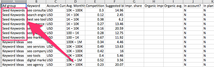
Let’s say I want to break down this list into just the keywords that have the word “tools” in them.

If I look manually, I have to sort through 700+ rows. I don’t want to do that.

Instead, I’ll use the Excel formula =IF to sort it for me.

First, I’ll remove the Ad Group column because I want to search all of them.

Then, I’ll add a “Category” column next to my search volume.

In the first available cell, I’m going to put the word “Tools” and then use the formula:

=if(isnumber(search(“tools,A12)),”Tools”)

Then, when a “tools” keyword is found in the first column (my keyword list), it gets put into the “Tools” category.

You can use this Excel SEO formula across your spreadsheets to put all of your keywords in certain categories.

This is a game-changer for SEO organization.

If you want only the keywords that contain the word “local,” for example, you could create a “Local” category.

This is a handy hack for organizing your keyword ideas for a fast search.

That way, if you’re working with a team of people who all need access to the same Excel file but for different reasons, none of your data gets messed up, and people still find what they need.

Moz has a good example of how this can be done for your spreadsheet data here.

To do this for all of your rows and columns, you can use a multi-cell ARRAY formula.

This spares you from inserting the same complex formula into every single cell of your spreadsheet.

Even if you don’t have 700+ cells to work with, it’s still a handy formula.

2. Create Pivot Tables for Spotting Data Outliers

Analyzing the data in your spreadsheets can be chaotic if there’s no organization.

Even when you can filter by categories, you might not spot outliers or “bad data” just by glancing at your list.

The good news is that Excel has an easy way for you to spot positive and negative trends in your data using pivot tables.

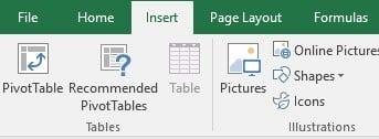
To create one, highlight a cell on your spreadsheet and click Insert > Pivot Table.

Next, you will see a dialogue box asking you to choose the data to analyze and where to place your pivot table.

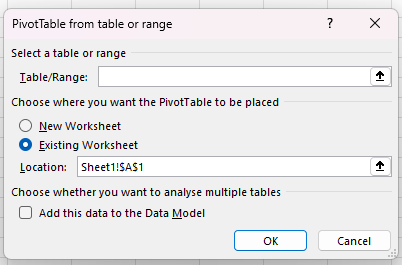
Your table gets automatically placed in the highlighted cell, but you can also create a new table or put it somewhere else from this box.

Once you’ve hit “OK,” you’ll see a prompt to choose fields to include in your pivot table.

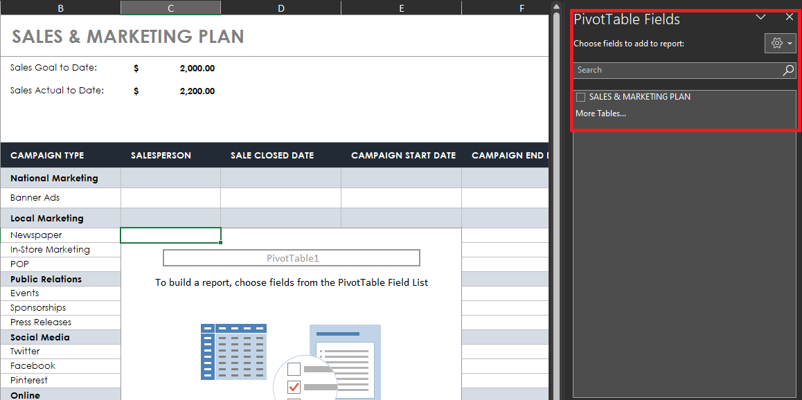
You can drag and drop fields wherever you need them, filter them, add columns, etc.

It’s completely customizable, so you can add or remove things later if needed.

You can use these tables for things like organizing links or URLs, grouping inbound links by DA/PA, keyword search per domain, or creating drop-downs for specific columns.

Here’s an example of what a functional pivot table might look like:

Not only does it organize your data in a more readable way, but it gives you several options for categorizing your data.

Pivot tables like this can be helpful if you’re using your keywords to inform your Google Ads strategy if you want to quickly spot high or low search volumes or cost-per-click (CPC) counts for specific keywords.

You won’t have to scroll up and down a list of hundreds of keywords to spot outliers.

And it looks pretty good, too.

3. Convert Volume Numbers Using “SUBSTITUTE”

There are plenty of different ways you can sort your data in Excel.

Finding the right option is key to productivity, however.

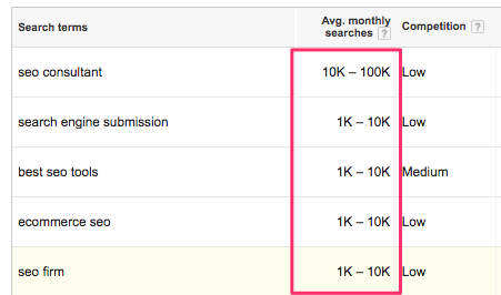
When you download data from a keyword tool, like Keyword Planner, the CSV files don’t always look pretty.

My keyword volumes, for example, look like this:

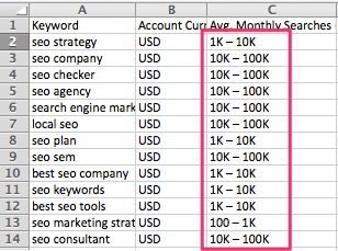
To be fair, they also look this way when I’m using Keyword Planner.

However, when I’m trying to search those volumes or organize them by the highest-to-lowest value, the format presents a bit of a problem.

Excel can’t sort my list based on terms like “10K” or “1M.” The M and K throw it off.

It needs real numbers.

Thankfully, Excel has a quick SEO formula to help you sort volumes properly.

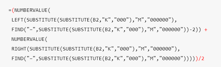
First, you want to replace the K and M and convert them into “000” or “000000.”

Create a new column called “Low to High” or something similar.

Select a cell in your new column, and insert =SUBSTITUTE:

Your formula should look something like this:

=SUBSTITUTE(C2,”K”,”000”)

The cell number changes depending on the row you’re converting.

Here’s what that looks like when you insert the formula:

The final results look like this:

You can also replace the M with “000000” using the same formula. It looks like this:

=SUBSTITUTE(C2,”M”,”000000”)

This should take care of all the Ks and Ms.

You can also do both at the same time (if you have a range of 100K – 1M, for example) using the following formula (replacing the cell number):

=SUBSTITUTE(SUBSTITUTE(C2,”K”,”000”), “M”, “000000”)

You can also use several formulas to find the minimum, maximum, and average search volume for your new column.

Here are the formulas for finding the minimum, maximum, and average:

Maximum:

Average:

Keep in mind that you might have to add additional columns to use these formulas, so make sure you label them properly.

You should be able to quickly discern between a high-to-low and low-to-high column without doing a lot of sorting or rearranging manually.

These formulas are supposed to save you time and energy, after all.

4. Format Title Tags With the “PROPER” Formula

Another tedious task you might have to do with your Excel SEO spreadsheets is reformatting your data.

Maybe you imported your title tags or keywords in a lowercase format, for example, but you want them capitalized.

You won’t sort through all your rows and columns capitalizing your text.

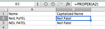
Or, at least, I hope you won’t because you can easily toggle lower and upper case characters in bulk using the PROPER formula, which looks like this:

=PROPER(C2)

Easy, right?

You want to create a new column and insert the formula there.

Here’s what that looks like:

The final result should be this:

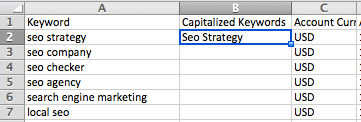
This works well if you have a lot of title tags you want to capitalize, too.

You can search for individual title tags using the HLOOKUP formula (which I’ll get to later).

You can also use the PROPER formula to reformat format names in all caps, even if your Excel SEO spreadsheet has upper and lower case characters.

You can use the UPPER function to change a lowercase keyword or title tag to uppercase (e.g., an acronym).

Here’s how that looks:

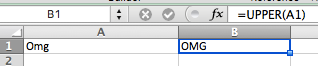
As you might imagine, the LOWER formula reverses the process.

Even though it’s a straightforward SEO formula, I’ve included it because many people forget about it, and it’s really useful for improving the presentation of your SEO data.

5. Search Large Spreadsheets With “VLOOKUP”

Some marketers like to segment their data into different Excel SEO spreadsheets.

You might have one for keyword research, one for emails, one for domains, etc., and sometimes you have all of that information in one place.

While having a large database of Excel SEO information is nice, it can be annoying to sort through all of those different columns, rows, or charts to find what you need.

As I mentioned earlier, if you have disorganized data, Excel’s search functions have their limitations.

And it’s even harder when you have data spread out over multiple rows and columns.

No worries, though, because there’s a formula for that (the Excel version of “there’s an app for that”).

You want to use the VLOOKUP formula, which looks something like this:

=VLOOKUP(A4;’Lookup Table’!A2:D1000;4;FALSE)

If you wanted to look up specific keywords between two sheets on the same spreadsheet, for example, it might look like this:

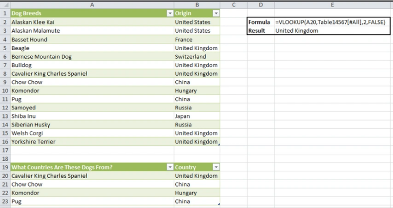
This SEO formula may seem complicated at first, but it gets easier once you break it down.

The first section is the name of the item you’re searching for. You’ll put it in quotes.

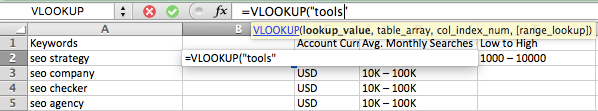
Next, you add your column range.

Then, you need to add a column index number. The first column in the range you’re searching is one, the second is two, and so on.

Since I’m trying to find keywords in the first column, I’ll go with one and follow it with a “TRUE” statement because I want an exact match.

I can also use “FALSE” if I don’t need an exact match.

Note that VLOOKUP only works if the data you need is in the first column (the left-most column) and the data is in ascending order (A-Z).

While you might need to format your columns before performing a VLOOKUP search, it’s still handy.

You can also use this for things like finding a product price or a specific category, like so:

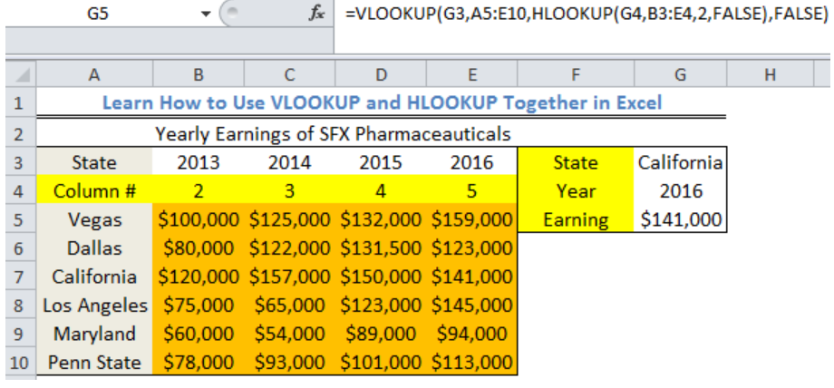
If you need to search rows, use the HLOOKUP formula instead. V is for Vertical search, and H is for Horizontal, like this:

An example HLOOKUP formula might be something like this:

=HLOOKUP(D3;’Lookup Table’!A1:D10;2;FALSE)

Click here for an example of the HLOOKUP function.

Both are quick ways of finding what you need, particularly if you need to search multiple rows, columns, or sheets within your document.

If needed, you can also use both features between two separate documents and search from drop-downs and pivot tables.

There are plenty of tutorials on using both SEO Excel formulas to find and calculate different data between sheets.

You can really become a pro at these two formulas if you want.

That’s why they far excel (no pun intended) the traditional search bar.

6. “XLOOKUP” to Find Specific Data Quickly

XLOOKUP lets you find specific data quickly. This makes it super-useful for looking for keyword rankings and search volumes.

This Excel SEO formula also allows you to look for exact or appropriate matches, and you can carry out searches based on multiple criteria, say for keywords or backlinks..

Here’s an example of an XLOOKUP Formula to find the keyword difficulty for the entry “google trends” from our spreadsheet below: =XLOOKUP(E3,A3:A13,D3:D13)

To use the XLOOKUP function in Excel, follow these steps:

1. Select the cell where you want to display the result of the XLOOKUP function (F3 in our example).
2. You’re going to type a keyword to search for in another cell (E3 in our example) and tell Excel to search for that from the keyword list in column A. So the first part of the formula is “=XLOOKUP(E3, A3:A13 which means check the value in cell E3 and look for it from column A.
3. Next, we want to find a value to return once Excel finds our keyword from column A. We’re looking for keyword difficulty so let’s build on the formula and tell Exel where to find that data range (it’s column D in our example) : =XLOOKUP(E3, A3:A13,D3:D13)
4. Remember to type a comma to separate the first argument from the second argument.
5. Type a closing parenthesis “)” to complete the formula.
6. Press Enter on your keyboard or click outside the cell to apply the XLOOKUP function and retrieve the result. The result should look something like this:

.

Remember to adjust the cell references and ranges according to your specific data and requirements when using the XLOOKUP.

7. Quickly Identify Duplicates Using “COUNTIF”

Not all of the data in your spreadsheet will be correct.

You’re going to want a quick, easy way to sort through it, remove duplicates, and move on with your day.

Excel’s formula for that action is COUNTIF, and it looks like this:

=COUNTIF(A:A,A2)

Let’s say you have a list of items in your first column (column A) that you want to check for duplicates.

First, create a new column and input the formula with the cell range from column A, like so:

Then, drag the fill formula to copy it to other cells, and you should see something like this:

TRUE indicates that multiples exist, while false means no exact duplicates exist.

This is a nice little SEO formula for searching keyword lists for duplicates because it only finds exact matches.

As you can see in the example above, even though the word “seo strategy” shows up at different times (seo marketing strategy, for instance), it’s not considered a duplicate.

If you want to highlight duplicates, you can do that with conditional formatting.

Click Home > Conditional Formatting > Highlight Cells Rules > Duplicate Values.

You can then select a color that you want your duplicates to have.

This is nice if you want to highlight them but are not ready to remove them.

If you want to remove them, you can do this by clicking Data > Remove Duplicates > Columns (just check or uncheck the columns where you want to remove the duplicates).

The process takes just a few minutes, and you can quickly clean up your data.

Some of these formulas can take some time to “master,” but Excel offers plenty of buttons and quick formulas to help you.

The COUNTIF formula is one of them.

8. Combine Data from Multiple Cells With “CONCATENATE”

CONCATENATE is a basic function in Excel.

It’s a time-saving tool for SEO Excel professionals and enables you to merge various columns into one.

Merging columns is useful if you’re managing large amounts of data, like keyword research, managing PPC campaigns, personalizing data for e-mail campaigns, and creating title tags.

Let’s say you want to create a personal greeting in an e-mail campaign using the person’s title and full name, you can use CONCATENATE to pull in data from separate columns in your spreadsheet to create a new column with both title and full name.

Using the CONCATENATE function in Excel, here’s the formula I used for the example above: =CONCATENATE(A3,” “,B3, ” “,C3,” “,D3)

Follow these steps to merge data from different column into one new one:

1. Select the cell where you want to display the combined data.
2. In the formula bar at the top of the Excel window, type “=CONCATENATE(” (without the quotation marks).
3. Enter the cell references or text strings that you want to combine.
   1. For cell references, type the reference of the first cell (e.g., A1).
   2. For text strings, enclose the text in quotation marks (e.g., “Hello”).
   3. You can include as many cell references or text strings as needed, separating them with commas and (“ “) for spaces in between.
4. Type a closing parenthesis “)” to complete the formula.
5. Press Enter on your keyboard or click outside the cell to apply the “CONCATENATE” function and combine the data.

To concatenate cells in Excel, you have a few options. Here’s a step-by-step guide on how to join cells using another method:

Using the TEXTJOIN Function (Available in Excel 2016 or Later)

The TEXTJOIN SEO Excel formula looks like this: TEXTJOIN(delimiter, ignore_empty, text1, [text2],

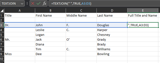
Here’s how to use it:

1. Select the cell where you want to display the combined data.
2. In the formula bar, type “=TEXTJOIN(” (without the quotation marks).
3. Enter the delimiter you want to use to separate the concatenated values. This can be a comma, space, or any other character enclosed in quotation marks (e.g., “, “).
4. Type a comma to separate the delimiter from the next argument.
5. Enter “TRUE” or “FALSE” to specify whether or not to ignore empty cells in the concatenation (TRUE to ignore empty cells, and FALSE to include them).
6. Type a comma to separate the argument from the next one.
7. Enter the first cell reference or text string you want to concatenate.
8. Repeat steps 7 and 8 for each additional cell or text string you want to concatenate.
9. Type a closing parenthesis “)” to complete the formula.
10. Press Enter on your keyboard or click outside the cell to apply the formula and concatenate the cells.

9. Average a Certain Metric With “AVERAGE”

Use the AVERAGE function in Excel to calculate the arithmetic mean of a range of numbers. It adds up all the numbers in the range and divides the sum by the count of numbers. This function is commonly used to find the average value of a set of data.

In SEO, the AVERAGE Excel function helps analyze your performance metrics like bounce rate, time on page, and conversion rates.

To use the “AVERAGE” formula in Excel, follow these steps:

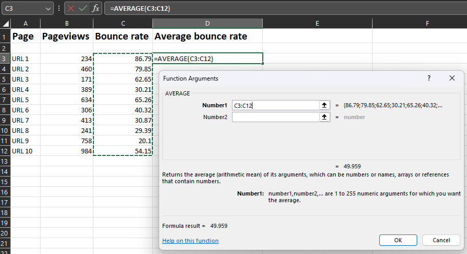
1. Enter your data into a column in Excel. For example, let’s say you want to find out the average bounce rate across a sample of URLs.

2. In an empty cell, type “=AVERAGE(” to start the AVERAGE formula.

3. Select the cell range containing the data you want to average. In this case, the cell range is listed under “Bounce rate.”

4. Close the formula with a closing parenthesis “)” and press Enter, or click ok from the dialogue box when prompted. You should see something like this:

Excel calculates and displays the average of the selected range of cells. This can be helpful for getting a quick average of a specific metric in your data set.

10. Check the Length of Your Text Data With “LEN”

Use the LEN or length function in Excel to calculate the length of a text string or the number of characters in a cell.

This Excel SEO formula returns the count of characters, including spaces and punctuation marks.

For example, if you enter =LEN(“What Is SEO? Search Engine Optimization Explained”)

Excel will return the length of the text, which is 49 characters.

It can be helpful for various reasons, including measuring the length of title tags and meta descriptions or analyzing the length of URLs.

You can also use LEN to calculate page content and measure character length. For instance, if you’re writing a meta description for online content, there may be a character limit. The best practice for the length of meta descriptions is around 160 characters. Let’s check a few samples using LEN:

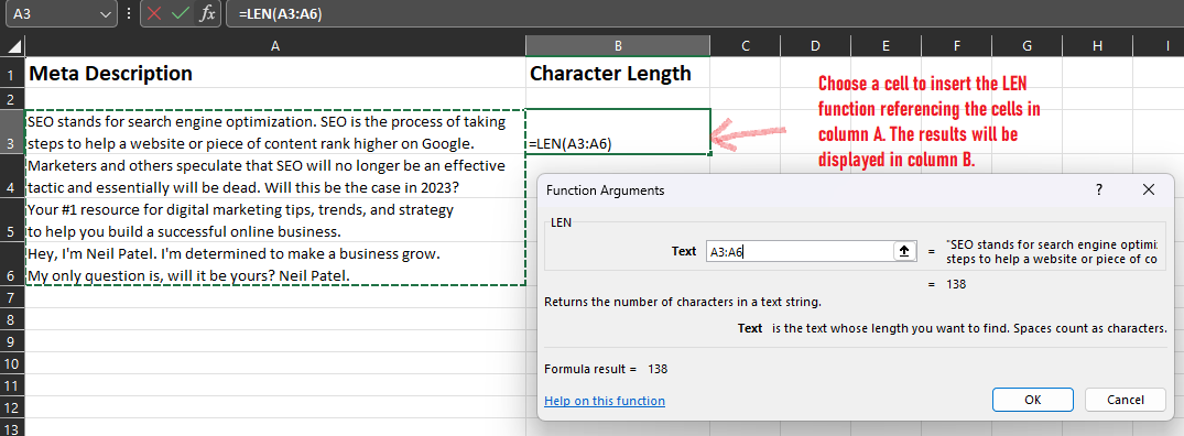
To check the length of your text data using the “LEN” function in Excel, just:

1. Enter your text data into a cell in Excel.

2. In an empty cell, type the formula “=LEN(” to start the LEN function.

3. Select the cell containing the text data you want to check.

4. Close the formula with a closing parenthesis “)” and press Enter.

Excel calculates and displays the length of the selected text data. The length includes all characters, including spaces and punctuation marks. Here is the result from our example:

11. Add a Series of Values With a Criteria Using “SUMIF”

The SUMIF function in Excel calculates the sum of values in a range that meets a specified condition.

It allows you to add values based on specific criteria or conditions. The function takes three arguments: the range to evaluate, the condition or criteria, and the range of values to sum.

Using the SUMIF function, SEO professionals can analyze and aggregate data, track performance metrics, and make data-driven decisions to optimize their SEO strategies.

It helps you summarize and understand data based on specific conditions, enabling more effective SEO analysis and decision-making.

As a simple example, let’s say you want to combine total shares from specific social media platforms as part of your SEO marketing analysis. You could add a series of values with specific criteria using the SUMIF function in Excel. Here’s how:

1. Identify the range of cells you want to evaluate based on the criteria. This range is typically called the “range” in the SUMIF function.
2. Identify the criteria you want to use to determine which cells to include in the calculation. This can be a number, expression, cell reference, or text. The criteria are typically called the “criteria” in the SUMIF function.
3. Identify the range of cells that contain the values you want to add based on the criteria. This range is typically called the “sum_range” in the SUMIF function.
4. Enter the SUMIF formula (=SUMIF(range, criteria, sum_range) in a cell where you want the result to appear.
   1. Range is the range of cells that you want to evaluate based on the criteria.
   2. Criteria are the criteria that define which cells will be included in the calculation.
   3. sum_range is the range of cells that contain the values you want to add based on the criteria. Data output from SUMIF for our example looks like this:

I pull out the values for Facebook and YouTube and add them together to display in column C using the following formula (select the cell in column C where you want the results then type the following into the formula bar:

=SUMIF(A3:A10,”Facebook”,B3:B10)+SUMIF(A3:A10,”YouTube”,B3:B10)

5. Press Enter to calculate the result. The cell will display the sum of the values that meet the specified criteria.

Note: The SUMIF function in Excel supports various criteria, including numeric values, expressions, and logical operators.

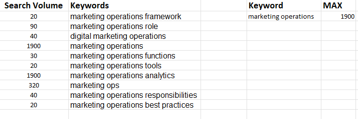
12. Find the High and Low End of a Data Set With “MAX” and “MIN”

Use the MAX and MIN functions in Excel to find the highest (MAX) and lowest (MIN) values, respectively, in a range of data.

Overall, Excel’s MAX and MIN functions allow SEO professionals to analyze and identify the highest and lowest values in various SEO-related metrics, such as performance, keyword research, content analysis, and URL optimization. These functions help in gaining insights, making data-driven decisions, and optimizing SEO strategies for better results.

Let’s say you want to check the maximum and minimum search volumes from a list of keywords related to marketing operations. The SEO Excel formula for checking the MAX might look something like this:

=MAX((A2:A13)

To find the highest and lowest values in a data set using the “MAX” and “MIN” functions in Excel, follow these steps:

1. Open your Excel worksheet and locate the range of cells that contains your data set.
2. Decide where you want to display the highest and lowest values. You can choose an empty cell or a specific location in your worksheet.
3. To find the highest value, enter the following formula in the desired cell:

=MAX(range)

4. Replace “range” with the actual cell range containing your data set. For example, if your data set is in cells A1 to A10, the formula would be:
5. =MAX(A1:A10)
6. Press Enter to calculate the result. The cell will display the highest value from your data set.
7. To find the lowest value, enter the following formula in another desired cell:

=MIN(range)

8. Again, replace “range” with the actual cell range containing your data set. For example, if your data set is in cells A1 to A10, the formula would be:

=MIN(A1:A10)

9. Press Enter to calculate the result. The cell will display the lowest value from your data set.

Using the “MAX” and “MIN” functions, you can easily identify the highest and lowest values in your data set without manually searching the entire range.

In addition, you can combine MIN and MAX with the INDEX function to pull out the respective keyword that matches your MAX or MIN value. Using the example above, here’s what you’de type as a function for the “Keyword” column (assuming your values are in column A):

=INDEX(B2:B11,MATCH(MAX(A2:A11),A2:A11,0))

13. Remove Spaces Before and After a Cell With “TRIM”

The TRIM function in Excel removes extra spaces from text in a cell. It removes leading, trailing, and excessive spaces between words, leaving only a single space between words.

TRIM is a simple Excel formula that looks like this: =TRIM(A1)

It’s useful for data cleaning and analysis, duplicate removal, and URL optimization (such as removing spaces in URLs).

Let’s say you have a list of URLs you want to check for spaces and have Excel remove those spaces. Here’s how you would go about doing that:

1. Create a temporary column for your updated URLs to be displayed in.
2. With the first cell of your temporary column selected, type “=TRIM(” (without quotation marks) In the formula bar at the top of the Excel window.
3. Select the cell or range of cells from which you want to remove the spaces. The cell reference will be automatically added to the formula as shown below:

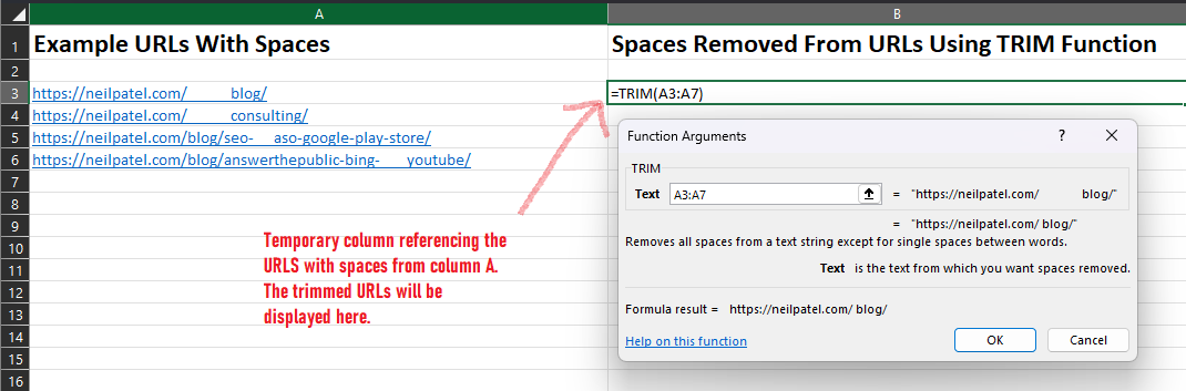
4. Press OK on your keyboard to apply the TRIM function and remove the spaces. Excel will then populate the temporary column with the URLs from column A with no spaces.

14. Change Keywords Between Uppercase and Lowercase With “UPPER” and “LOWER”

The UPPER function converts all letters in a text string to uppercase, while the LOWER function converts them to lowercase.

By utilizing the UPPER and LOWER functions in Excel, SEO professionals can effectively format and standardize text, analyze keyword data, optimize URLs, and ensure consistency in content.

To use it, press Select a blank cell to apply the “UPPER” or “LOWER” function, include the reference to the cell you want to change, then hit OK to change the case.

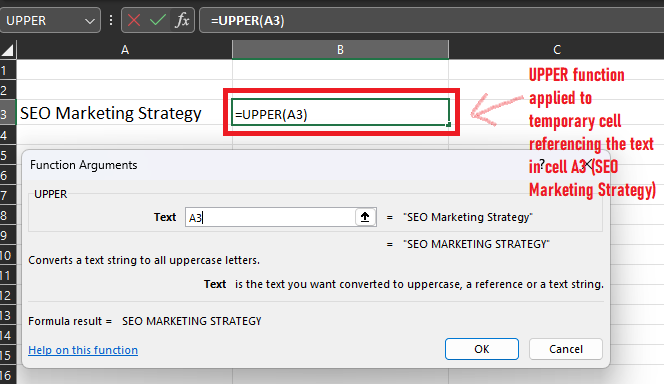
You should see something like this:

All you have to do then is copy the converted case from column B and use it to replace the text in column A using copy and paste.(Right click the text in column B, select copy, select cell in column A, right click and choose paste). You can then delete column B.

The “UPPER” function converts the text to uppercase, while the “LOWER” function converts the text to lowercase.

That’s just a single cell, it’s likely you’ll have more entries in your spreadsheet, so here’s an how you would apply UPPER or LOWER to more than one cell:

Suppose you have a spreadsheet with ideas for blog content, and want to convert the headings into upper or lower case. Follow these steps:

1. Create a temporary column where your case conversions will appear.
2. With the temporary column selected, type “=UPPER(” (without quotation marks).
3. Select the cells with the text you want to convert (highlighted in blue below).
4. You will see the function bar automatically populates values in the highlighted cells (A3:A10 in this example).
5. Press OK when prompted, and your temporary column will update to reflect the case conversions.

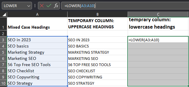
The cells will now display your blog title headings in uppercase. Keep the column as is, or copy and paste them over to replace the contents of the original column (mixed case headings).

Similarly, if you want to convert the text to lowercase, use the “=LOWER(” formula instead of “=UPPER(” in step 2. (Shown in column C above).

15. Scout Out Errors With “IFERROR”

The IFERROR function in Excel handles errors that may occur in a formula.

It allows you to specify a value or action if an error occurs in the formula and prevents it from disrupting the entire spreadsheet.

This function can enhance the reliability and accuracy of Excel SEO processes, ensuring that errors do not disrupt data analysis, reporting, or other SEO-related tasks.

To use IFERROR, enter the following formula:

=IFERROR(VLOOKUP(D2,$A$2:$B$12,2,0),”Not Found”)

To scout out errors with the “IFERROR” function in Excel, follow these steps:

1. Select the cell where you want to display the result or error message.
2. In the formula bar at the top of the Excel window, type “=IFERROR(” (without the quotation marks).
3. Enter the formula or expression that you want to evaluate for errors.
4. Type a comma “,” to separate the formula from the value or message you want to display if there is an error.
5. Enter the value or message you want to display if there is an error.
6. Type a closing parenthesis “)” to complete the formula.
7. Press Enter on your keyboard or click outside the cell to apply the “IFERROR” function and scout out errors.

FAQs

Conclusion

Plenty of people don’t like using spreadsheets or messing around with Excel SEO formulas.

I get it.

Some of the formulas are a little complicated and bulky to remember.

However, if you’re using spreadsheets—especially Excel spreadsheets—for SEO or marketing research, you should really brush up on some formulas.

More specifically, look at ones that will help you quickly search or clean up your data, like VLOOKUP and COUNTIF.

Converting your volume numbers using SUBSTITUTE is a must for keyword research.

And learning how to create more complex (but helpful) things like pivot tables saves you so much time and energy in the end.

SEO is complicated enough as it is and being efficient with SEO is vital.

Ease the burden by learning a few Excel SEO hacks in the process.

To make things easier, I’ve prepared a bunch of SEO report Excel templates, spreadsheets, and worksheets. Alternatively, take a look at how my team at NP Digital is using Excel and more to power efficiency.

What Excel SEO hack do you use for cleaning up your spreadsheets?